We have made a folder in the server space for Representation AK 3, called "Inlämning" ("/ak3/A31REA Representation 3/Inlämning"). For submitting your work, create a folder in "Inlämning" and name it anything you want. The folder should contain:
-A text file (.txt or .rtf) called "medlemmar", with the names of the members of the group (very important, otherwise it is going to be difficult to know who has done what!).
-2 to 4 pdfs of your A3s (diagrams, maps…).
-A folder called "Modell", in which you should include pictures of your model (from 1 to 5 pictures should be enough) .
There is an example folder conveniently called "Example", if you wonder how your submission could look like. You can also copy-paste that folder and fill it in with your information.
This material will be only for evaluation and administrative purposes. We are contemplating the idea of showing some of the work to the rest of the school (we will ask for your permission beforehand), so don't throw away your models!
Open Street Map into QGIS.
 |
| From Open Street Map. CC BY SA 2.0 license. |
Getting and using Open Street Maps in QGIS.
Some of you have asked if there was possible to get maps into QGIS. Besides inputing files from other maps services, the Open Street Maps database is a good source for maps, even if sometimes they may be incomplete. Open Street Maps is a collaborative project to create a free editable map of the world, with a database available through the Creative Commons Attribution-ShareAlike 2.0 license . It is under development, so not all areas are covered with the same amount of detail, but many parts of Europe are quite reliable, and you can even get data from other areas in the world. The best thing is that it is free and that all material is provided with a very liberal license (CC BY-SA 2.0). You can also download images of maps, etc (Google Maps seem to have a much more restrictive license, check point 10.1.3).
There are two ways we have found to get the data into QGIS:
A. The easy one, but limited data:
1-Download shape files of Open Street Maps from cloud mate ( http://downloads.cloudmade.com/europe/northern_europe/sweden#downloads_breadcrumbs). You can download many parts of Sweden (Stockholm among others), the whole Sweden, and many other parts of the world (http://downloads.cloudmade.com) so this may be useful for future projects. Remember to download the files that are called shapefiles, like this one for Stockholm http://downloads.cloudmade.com/europe/northern_europe/sweden/stockholm/stockholm.shapefiles.zip
2- Unzip them, and you can open them in QGIS (either by clicking the files with ".shp" extension or directly from QGIS, with "Layer > New > New Shapefile Layer" in the menu bar, for example). They will come up distorted, because of the coordinate system of the file. If you wonder what the coordinate system is, and how important is the history of representation, check this http://en.wikipedia.org/wiki/Map_projection).
3- You can change the coordinate system to any other you want, for example "Google Mercator", which is the same that Google Maps uses. You can do this by going to "Settings > Project Properties" and selecting the "Coordinate Reference System (CRS)" tab. There "Google Mercator" is under "Projected Coordinate Systems > Mercator > Google Mercator". Check also the box that says "Enable 'on the fly' CRS transformation", and press OK.
That was that.
You can go now and "Open Attribute Table" on the layer (by right clicking on it) and select data according to the table. As you can see the amount of data is limited, though substantial (if you include all the shapefiles), and it will allow you to match any data with the map of Stockholm.
B The proper way, though complicated.
For having access to all Open Street MAp information you will need to install a database in your computer, that you will access through QGIS. This involves installing some software and using the command line. I had a bit of trouble doing this, but I finally managed. Here is a tutorial for MAC:
We had problems installing PostGIS (if you try to create a database as explained in the tutorial and "template_postgis" does not show as an option in "Template" , you have the same problem). To fix the problem, You can try to find where the installation zip for PostGIS is in your computer, or download it from here:
and run it. Then follow the steps as indicated in the rest of the tutorial (download osm2pgsql … etc). You also have to enable to save your password when you start the server in pgAdmin III.
You can fins another tutorial with even more advanced style editing explanations here.
Heights Applet update.

We have updated the heights applet for those of you that may want to use it in the project (or in the future). The new applet works exactly as it did before, with a couple of added features:
1. Smoothing:
Now the applet has a smoothing spinner, set by default to 0 (no smoothing, as before). If you move the slider to a number larger than 0, you will see how the heights even out (with a very large number the surface will become basically flat). The Smoothing is a bit similar to that used in the google ngram viewer that we have shown as an example in the course. As you may see in that example, the smoothing gets rid of "noise" (big differences in the samples) at the expense of detail. The more you smooth, the easier it is to see general trends, but the more difficult it is to see specific events. The smoothing, both in the Ngram Viewer and in our applet works by averaging the value of each sample point with those around it. One can select how many samples around are going to be used in the averaging (this is the number that appears in the smoothing spinner box).
For the smoothing (http://en.wikipedia.org/wiki/Smoothing) the applet uses a formula for adding up and averaging the values of adjacent squares which is called a "Gaussian Convolution Filter" . This is basically the same Gaussian Filter that you may have used in Photoshop, to reduce noise in images. What the smoothing spinner does is to specify the amount of neighbor to each square cell that are going to be used to average values: 2, for example, means that it will average all the squares around each cell that are within 2 squares to the right and left and 2 squares up and down (2 square distance in x and y), using the gaussian formula.
If you do horizontal sections now (height curves or isolines, as they are also called) you will get much nicer looking curves also.
2. Frame:
By default the applet calculates the bounding box for the data (the smallest rectangle in which the data fits), and then it scales the grid accordingly. If one uses different sample data it may be difficult to compare them, since they will produce grids that are placed and scaled differently, even if they overlap . To solve this it is possible now to have a layer called "FRAME" (or "frame", capitals don't matter ) that the program will use for making the bounding box. It will ignore otherwise the data in that layer (it won't count any polygon in the layer when calculating areas, for example), so don't put any data that you want to use on that layer! (see the examples included).
Here is the applet:
We have put some sample data with the "frame" layer on also:
The applets are also under the Applets column on the right.
Spacematrix, Meta Berhauser Pont.
 |
| Spacematrix, Meta Berghauser Pont and Per Haupt. |
I hope everyone enjoyed Meta Berghauser's lecture as much as we did!
Meta has kindly given us a copy of her presentation so you can have another look at it, here. We have also ordered the Spacematrix book at the library. And here are also a couple of links to her work, that she showed during the lecture (we have added the links also to the software list on the right):
Gisdro
The co-researchers of the Rotterdam project that is presented by Meta Berghauser Pont should be mentioned in the presentation. The co-researchers are Akkelies van Nes (assistant professor, TU Delft) and Bardia Mashhoodi (PhD candidate, TU Delft). Furthermore, Per Haupt should be mentioned as the co-author and co-researcher of Spacematrix.
The co-researchers of the Rotterdam project that is presented by Meta Berghauser Pont should be mentioned in the presentation. The co-researchers are Akkelies van Nes (assistant professor, TU Delft) and Bardia Mashhoodi (PhD candidate, TU Delft). Furthermore, Per Haupt should be mentioned as the co-author and co-researcher of Spacematrix.
Main Task
Now is the time to start with the final and main task. During these first weeks we have been trying out a couple of examples of visualizations, using heights to represent values, and isovists to define viewing areas. During the next weeks you will either use one of the examples explained (heights or isovists), or if you feel like it propose your own form of visualization. You will use this within your design projects, that is, you will use information or a problem that may be interesting to look at from your main design course. Remember anyway that we will not be evaluating your project, but only your contribution to the representation course.
Schedule:
Besides the scheduled lectures we have scheduled tutorial times, they are in the calendar (link on the right column of this blog). If any of you have problems with the dates we can surely find some way around it. I (Pablo) am also at the school most of the days, and you can always pass by my office (C 304, on the 3rd floor) if you have any doubts or need advice.
Review and material:
We have scheduled a final review the 25th of November. Then you will present all the deliverables(specified below), and we will tell you how to improve them for the final delivery date, January 13th, 2012. We have also scheduled a final tutorial day the 9th of December, after our final review to help you out with this.
Deliverables.
A physical model, A3 size in base.
Between 2 and 4 A3s (depending on your project).
Groups:
The work will be carried in the same groups you have formed. If you want to change your team (there were some cases in which these groups were provisional) just drop us a mail (pablo.miranda(AT)arch.kth.se).
We will keep you updated (how to book times for the tutorials, etc) during the coming week.
Lecture Diagrams in Architecture

To follow up on my lecture Diagrams in Architecture I provide you hereby the diagram of the lecture itself. Please review the following books and essays that were referred to in the lecture:
- The Diagrams of Architecture by Mark Garcia, book
- Parametric Diagrammes by Patrik Schumacher, essay
- What is a diagram anyway? by Anthony Viddler, essay
- Move by UNStudio, book
- The Future of Information Modeling and the End of Theory, Less is Limited, More is Different by Cynthia Ottchen, essay
Sander
Isovist using Grasshopper in Rhino
 As I showed some of you last time it is possible to do an (almost) interactive Isovist directly in Rhino using the plugin Grasshopper. This means that you can move around a point and the Isovist will update. Similarly changing the obstacles will also update the Isovist interactively (much like the Java applet which Asmund demonstrated last time). I have put together a small demonstration of this which you can download in the applets section of the blog or here.
 Grasshopper is a free plugin (download) for Rhino that will only run on a PC (that means running bootcamp if you are on a Mac) where at least Service Release 8 for Rhino is installed. A workaround is to download the Rhino trial version which comes with Service Release 9. This version will only let you save 25 times on the Rhino side of things though.
Please note that this is NOT a part of the exercise and also that I WILL be doing a demonstration of how this all works Friday 14/10/2011. Happy Isovisting!
-Anders
Please note that this is NOT a part of the exercise and also that I WILL be doing a demonstration of how this all works Friday 14/10/2011. Happy Isovisting!
-Anders
Excercise 2: Isovists
In the second exercise we will generate new spatial descriptions, in the form of diagrams, from urban plans. As an example of this we will focus on a projection technique called isovist or view-polygon, the isovist is usually defined as the area (or volume in 3D) that can be seen from a single point in an environment. It can be geometrically constructed, or it can also be approximated in a physical model with a point-like light source. In the previous exercise we saw how we could use the z-axis to represent and visualise additional information (a magnitude of some sorts), and in this exercise we will use the z axis to show changes over time (moving along a path), or an ordering of shapes according to area.
We have made another applet for you to work with.
The applet takes a DXF as input with the following information:
- Non-intersecting Lines or Polylines (open or closed) on a layer called "obstructions".
- Circles on any layer will be interpreted as view points (optional).
- A single Polyline on a layer called "path" (optional, if present will override the points).
And you can export a DXF with the following data:
- All obstructions as Lines.
- View points as Circles.
- Path as Polyline.
- Isovists as closed Polylines.
Number of Samples: When working with paths you can decide the number of total samples along the path for the calculations.
Vertical Scale: All the isovists are visualised stacked on top of each other and you can set the z distance between each "layer".
Calculate isovists: You need to press this for anything to happen after you import a file, or if you change the number of samples.
Submission:
-Use the A3 Adobe Illustrator template, (downloadable from "Templates" on the blog) for submission.
-Submit your drawing to ak3/A31REA Representation 3/Övning_2
-You should submit before October 21st.
Updated Heights Applet

We have updated the applet for transforming densities of points (represented as circles in the dxf file) and areas (as polygons in the dxf file), after the testing last week. Now it should be possible to rotate in windows (hurray!) and to load and save a file from anywhere (so you don't have to copy it into the same folder as the applet). There are also a few other improvements to make it more robust and just a slight change in the visualisation. Hopefully more changes and improvements will be introduced as we test and use it. You can download the new version from here or from the Applets tab on on the right. It does not run properly on the "Datasalen"due to permissions that need to be set by the administrators, but if there is a big demand for this we can ask them to fix it.
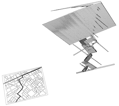
Exercise 1: Contours and Heights, adding an extra dimension to information.
 |
| Stan Allen, "from Object to Field". |
We are going to test a few ways of visualizing data. The data we have for testing is made of polygons or points. This data could be anything you may draw and map from any of your projects: cigarette buts on the floor, events on a part of the city, trees on a park, cars parked, lampposts… as long as they are represented by points or polygons anything could be our data. The points and polygons we have are originally from a GIS database (links are giving under "Resources" on this blog) of Stockholm, though we won't concentrate that much on the meaning of this information at this point. We will use them just to check techniques, later in the course we will use these techniques with data that may be meaningful to your project.
We will explain how to use this sample information, and how to process it through a small application or APPLET that we have developed for the course (downloadable at "Applets", on this blog).
The actual task, consist in producing a drawing from the data sets (the drawing could show one data set, or a comparison of different data sets, for example). The drawing should identify some important feature or pattern in the form the data set is represented: a boundary, a gradient (a direction of steepness, check the lexicon on the blog), valleys, holes, peaks… Use the chance to learn how the representation system works, test different ways of manipulating and analyzing it in your favorite modeling or CAD package. Be selective of the information you present, don't crowd too much information together, be clear and precise.
Some of the techniques you can use to represent these features :
-Boundary lines (boundary contour).
-Vertical Sections.
-Contour lines.
-Meshes and wireframes.
-You can download some test datasets formatted as dxf under "applets", from the blog, there are some more on the server space: ak3/A31REA Representation 3/Datasets.
Submission:
-Use the A3 Adobe Illustrator template, (downloadable from "Templates" on the blog) for submission.
-Submit your drawing to ak3/A31REA Representation 3/Övning_1
(it seems that the directories have been renamed, I have updated the references), as indicated in the "Server Space" post from last week.
-You should submit before the next day we meet, October 7.
Network Analysis Software
Some of you wondered last Friday where would be possible to get some software that does spatial network analysis, as those done through Space Syntax methods. Here are a number of suggestions from some of my researcher colleagues:
-Webmap-At-Home: this is a simple but useful program, free to download that does Axial Analysis. It has been developed by Sheep Dalton, one of the key figures behind Space Syntax. I have added a link to it also in the Software list on the blog.
-AJAX for Windows developed at CASA, UCL.
-There are a number of other software (some old, some commercial or related to commercial products) here.
-There are also a number of licenses at the school for using PSD (Place Syntax, developed here at KTH Architecture) and Mapinfo. As far as I know they are installed in some of the computers closer to the door in the computer lab. Since not many people use them, you should ask the IT people if you find any problems, if anyone wants to give it a try. You can also ask me, and I can redirect you to someone that knows how to use it and set it up.
Discourse: James Corner and Stan Allen

As you have probably noticed we have started to add more and more links here to the blog. We would encourage you to explore them all. To help you along here are a few words and links on two of the key people mentioned in the Discourse section. James Corner and Stan Allen are both practicing architects and theorists working out of New York City. They were co-directors of the studio Field Operations but have since parted ways, leaving Corner to run the studio and Allen to start up his own studio Stan Allen Architects.
As theorists, lecturers and writers their way of representing the city and the methodologies they have developed in response to this have been quite profound in shaping new ways of mapping, visualising and unfolding the complexity of the city. Besides their academic output Corner has been involved in designing the NY Highline project with Diller & Scofidio and Allen has been noted for a number of smaller scale projects. We would encourage you to pay particular attention to the following articles and essays:
The Agency of Mapping: Speculation, Critique and Invention by James Corner
Field Conditions by Stan Allen
Diagrams Matter by Stan Allen
- Anders
- Anders
Update: The James Corner link appears to be dead. I have not been able to dig up a substitute link, but perhaps some tenacious Googling could yield some results!
Research task
As mentioned this morning the idea with this first small task is just to get started checking some references and shearing your findings with the rest. To recap a bit on what to do:
-If you don't have any group yet from your main design project, make a temporary one for the first tasks (you can change later when the task from Representation gets more tightly related to your design work and the group you may have there). Groups should be 3 people, max 4.
-There is a list of themes to research ( by searching online, checking the library...) on the studio space, by the wall on the corridor. Choose one (write the name of your group by it). If there are no available ones, or if you are really interested on a subject that some one else is also looking at, more than one group can choose a subject.
-On the blog there is an Adobe Illustrator template (an A4 format with the file extension .ai) under Templates. If you don't have a copy of illustrator, you can download the Open Source and free program Inkscape (there is a link on Software, and I have checked that it works to open the template on it, at least in Mac). Mac versions of Inkscape are a bit buggy, from my experience, but usable. If you don't know how to use a vector graphics editing program, such as illustrator or Inkscape, this is a good chance to have a go at it! it will be very useful for doing layouts an reworking your drawings and diagrams in the future.
-The template has some test text and some advises for using it. It basically says that if you copy text or images, you should mention the source. This is not only right and proper, but useful for anyone else that may want to check where you have found stuff.
-When you are done, submit a copy of your Research task to the KTH Server, as explained on the previous blog entry. Name it like this: G+number + _ + name of reseach task.pdf (yes, export it or print it as pdf from Illustrator or Inkscape). The file could then be called something like this: "G03_SpaceSyntax.pdf" or "G12_GIS.pdf", that would be research on space syntax done by group 3, or research on GIS done by group 12.
-For getting the number of your group, just send me an email with the people in it, and I will give you a number.
We can then print them (I can do that since I guess it is easier) and have them all placed on the studio space, so you can all check also what the rest of the people have looked at. Do this before next time we meet, that is Friday the 23rd.
Good luck!
Server space
Hej Allihopa, och tack för idag.
Here is a some information about the space in the server for Representation AK3, and how to access it.
There is a directory/folder at KTH Arkitektur server that we will use for the whole course, for sharing large files and submitting your work. All exercises we do should be submitted there.
The directory for the course is:
ak3/A31REA Representation 3
and the one in which you should submit the results of your research task is:
ak3/A31REA Representation 3/Research Task
How to login:
You should be able to access the folder when you are logged in in a computer from the school (talk with the IT services otherwise). From outside the school or a wireless connection you should be able to access it through any sftp client. I use Filezilla, which is free and open source. You can download it here:
http://filezilla-project.org/
download the client (we have added a link under "software" in this blog, there on the right, at the bottom).
Install it for your platform, and where it says Host fill in (without quotation signs)
"sftp://login.arch.kth.se". You may also need to specify the port, which is 22. Username and password are the ones you use for you login at the schools computers (not the one you use for your KTH webmail, if they are different). If you have any problems with this you should as IT services for some help.
The Blog
Välkomna allihopa till Representation kursen för AK3. Vi ska använda bloggen för att lägga till information, referenser, osv. Vi ska träffas först den 16 september, Fredag, klockan 9:00. Ve ses då!
Representation.
During the course we will focus on geometric methods of representations that will allow us to handle information and descriptions of form at an urban scale. The objective of the course is to learn to represent and manipulate attributes characteristic of the larger architectural scale of the city and landscape. We want also to answer to recent trends and developments in relation to working at these scales, such as the increase of information available at urban and regional size, and the development of computational methods of analysis of urban morphology and space.
During the course we will look at two main techniques, that will be introduced during the first weeks through a number of exercises. These techniques will later be informed by material and data from the parallel design course. The first technique is based on the conventions for representing values on a 2 dimensional surface, through contour lines and height maps, as used in meteorology, social sciences, engineering, and cartography. The second techniques is based on the principles of projection, and will focus on drawing a type of diagram known as a shadow volume or isovist.
During the course we will look at two main techniques, that will be introduced during the first weeks through a number of exercises. These techniques will later be informed by material and data from the parallel design course. The first technique is based on the conventions for representing values on a 2 dimensional surface, through contour lines and height maps, as used in meteorology, social sciences, engineering, and cartography. The second techniques is based on the principles of projection, and will focus on drawing a type of diagram known as a shadow volume or isovist.
Subscribe to:
Posts (Atom)